Theoretical notes

This chapter presents the theoretical background of the program: active and passive earth pressures, loads on the backfill, groundwater, seismic actions, LEM and FEM methods, anchors and checks. The same text is included in the computation report.

Introduction

The bulkheads are civil engineering works that find application in a lot of problems related to the stabilization of slopes or supporting ground embankments. They are also used for the mooring of large vessels, or to shore up the walls of trenches and other excavations or to realize sealed caissons for underwater works. So a great importance must be given to the design of such a work, particularly as regards the structural and geotechnical design. As regards the calculation is worth pointing out that there aren’t, to date, the exact computation methods, and this is also due to the complex interaction between the depth of excavation, the stiffness of the material constituting the bulkhead and the resistance due to passive pressure. In any case, the methods currently used can be classified into two categories:

1. Methods that are based on a discretization of the bulkhead model (finite difference or finite element).

2. Methods that rely on simplistic conjecture in order to face the problem with the simple study of equilibrium of a rigid body.

Between the two classes of methods exposed to the previous list, the finite element method is the most rational, since it is based on considerations that involve both the static problem (equilibrium) and kinematics (consistency).

Types of bulkheads

The types of bulkheads most used at present can be classified as follows:\ 1. Bulkheads in reinforced concrete\ 2. Timber sheetpiling\ 3. Steel sheetpiling

Bulkhead analysis

Some preliminary considerations

The elements that contribute to the calculation of a bulkhead are various. In fact are involved concepts related to the flexibility of the piles, the calculation of the embankment thrust, the stiffness of the soil etc. Observe the following figure:

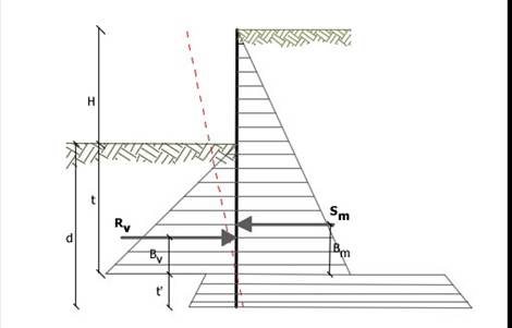
Figure 1: Scheme of pressures acting on the bulkhead

It can be seen that the lateral pressures which are called to participate in the equilibrium are the active pressure developed on the reverse side of the bulkhead and the passive pressure which develops in the front of the bulkhead (downstream of the bulkhead). The calculation, in the context of simplified methods or numerical methods, of the thrust on the reverse and downstream of the bulkhead is usually conducted either by the method of Rankine or with the method of Coulomb. It notes, however, that the method of Coulomb provides more accurate results because the bulkhead being a work usually flexible and thus showing more movements is generated friction at the interface bulkhead-ground that can be taken into account only through Coulomb’s thrust coefficients.

In using the finite element method it also must be calculated a ground reaction coefficient, ks, as well as the active and passive ground thrust. If it comes to analysis in undrained conditions it is also necessary to know the value of undrained cohesion. It also important to consider that if you want to be duly taken into account the friction between the soil and the work you must know of the angle of friction between the ground and work (in fact). In conclusion the parameters (in terms of ground properties) which must be available to perform the analysis are the following:

1. Ground angle of internal friction

2. Ground cohesion

3. Ground unit weight

4. Friction angle between ground and material that constitutes the work

Computation of active thrust

The active thrust can be calculated using Coulomb’s method or alternatively using the Theory of Caquot.

Coulomb’s method

Coulomb’s method is able to take into account the most significant variables, especially with regard to the frictional phenomenon that is generated at the bulkhead-ground interface. For homogeneous and dry ground, the pressure diagram shows linear distribution (measured at the depth z):

The total thrust, which is the integral of the previous relationship on all the height, is applied to 1/3 of H and is calculated using the following expression:

Having indicated with k_a the value of the active pressure coefficient, determined with the following relationship:

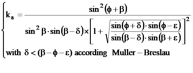
γ_t = ground unit weight

β = inclination of the inner wall of the horizontal plane passing through the foot

φ = soil angle of shearing resistance

δ = soil-bulkhead friction angle, positive if counterclockwise

ε = inclination of the ground level of the horizontal plane, positive if counterclockwise

Caquot’s method

Coulomb’s method appears to be a sufficiently accurate method for the evaluation of pressure coefficients at limit state. However is affected by the hypothesis concerning the planarity of the sliding surface. This hypothesis is removed by applying the theory of Caquot which is based on the use of a sliding surface in the shape of a logarithmic spiral. According to this theory the active pressure coefficient is determined using the following formula:

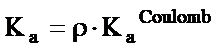
Where the symbols have the following meaning: - K_a^Coulomb is the coefficient of active pressure calculated with the theory of Coulomb - ρ is a multiplicative coefficient calculated with the following formula:

The symbols are calculated with the following formulas:

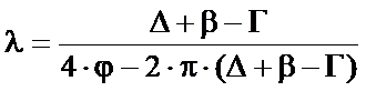
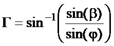
The symbols have the following meaning (see also figure below): - β is the inclination of the upstream profile measured compared to the horizontal - φ is the angle of internal friction of the pushing ground - δ is the friction angle at the work-ground interface

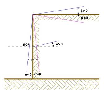
Figure 2: Convention used for the calculation of the pressure coefficient according to the theory of Caquot

Uniform load on the embankment

A load Q, evenly distributed on the ground surface induces constant pressures equal to:

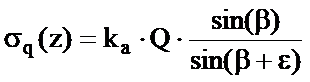
By integrating the stress indicated in the above formula we obtain the total thrust due to overload:

With application point to H/2 (stress distribution constant). In the above formulas the symbols have the following meaning:

β= Inclination of the inner wall with respect to the horizontal plane passing through the foot

ε= Inclination of the ground level with respect to the horizontal plane, positive if counterclockwise

ka= Active pressure coefficient calculated in the previous paragraph

Strip load on inclined ground level

The acting load is decomposed into a tangential load and a perpendicular load to the embankment, the pressure induced on the wall will be calculated as shown in the two paragraphs that follow.

Strip load perpendicular to the plane of action

A load partially distributed by initial abscissa x1 and final abscissa x2 generates a pressures diagram on the wall whose values were determined according to the formula of Terzaghi, which expresses the pressure to the generic depth z as follows:

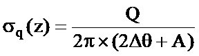
With:

Δθ=θ₁-θ₂;

A=sin(2θ₁)-sin(2θ₂)

B=cos(2θ₁)-cos(2θ₂)

θ₁=arctg(z/x₁)

θ₂=arctg(z/x₂)

By integration we will get the result and the relative arm.

Strip load tangential to ground level

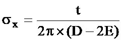
T= Load intensity [F/L²]

D= 4·log[sinθ₁/sinθ₂]

E= sin²θ₁-sin²θ₂

Load lines on the embankment

The load lines generate an increase of pressure on the wall that, according to Boussinesq, at the depth z, may be expressed as follows:

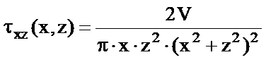
Where the symbols have the following meaning:

V= Load intensity expressed in [F/L]

X= Distance, in horizontal projection, of the load application from the wall

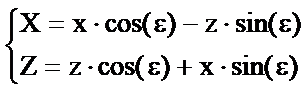
If the action plan is inclined by ε the reference system xz is rotated in XZ, through the following transformation:

Thrust in the presence of ground water

The groundwater with surface distant Hw from the base of the structure, induces hydrostatic pressures normal to the wall that, at the depth z, are expressed as follows:

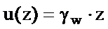
The total buoyancy is obtained by integration over the whole height of the previous relationship:

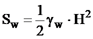
Having indicated with H the total height of thrust and with γw the unit weight of water. The thrust of the ground is obtained by replacing γt with γ't (γ't = γsaturated - γw), specific weight of the material immersed in water. In seismic conditions the thrust exerted by water is evaluated as follows:

applied to 2/3 of the height of the water table H_w [Matsuo O'Hara (1960) Geotecnica , R. Lancellotta]

Effect due to the presence of cohesion

The cohesion induces constant negative pressures equal to:

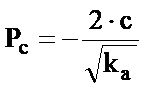
It is impossible to determine in advance what is the decrease induced by the thrust due to cohesion. It was calculated the critical depth Zc as follows:

Where the symbols have the following meaning:

Q= Load acting on the embankment eventually present

γt = Soil unit weight

β = Inclination of the inner wall of the horizontal plane passing through the foot

ε = Inclination of the ground level of the horizontal plane, positive if counterclockwise

C= Material cohesion

k_a= Coefficient of active pressure, as calculated in the previous steps

If Zc, calculated with the above formula, is less than zero, it is possible to directly superimpose the effects of the diagrams, by imposing a decrease in the original thrust diagram calculated as follows:

Where it is indicated by the symbol H the height of the total thrust.

Earthquake

Active thrust in seismic conditions

In the presence of earthquake the calculation strength exerted by the embankment on the wall is given by:

Where the symbols have the following meaning:

H= excavation height

k_v= vertical seismic coefficient

γ= soil unit weight

K=total active thrust coefficients (static + dynamic) (see Mononobe & Okabe)

E_ws= buoyancy of water

E_wd= hydrodynamic thrust

For impermeable soils hydrodynamic thrust Ewd = 0, but a correction is made on the computation of the angle β in Mononobe & Okabe formula as follows:

In soils of high-permeability under dynamic conditions continues to apply the above correction, but the hydrodynamic thrust assumes the following expression:

With H' height of the water table (shown in the section concerning the calculation of buoyancy).

Passive resistance

For the calculation of the passive resistance may be used the two methods used in the calculation of the pressure at active limit state (Coulomb’s method and method of Caquot).

Coulomb’s method

For homogeneous soil the pressures diagram under passive limit state conditions is linear with law of type:

By integrating the previous relationship on the height of thrust (which for the bulkheads must be carefully calculated) we get the total passive thrust:

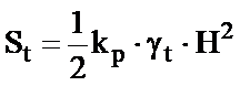
Having usual indicated with H the thrust height, γt soil unit weight and with kp the passive pressure coefficient (under conditions of passive limit state). The value of this coefficient is determined with the following formula:

With values equal to: δ\< β-φ-ε (Muller-Breslau).

Method of Caquot

The method of Caquot differs from Coulomb’s method by the calculation of the pressure coefficient at passive limit state. The coefficient of passive pressure is calculated, with this method, by interpolating the values in the following table:

Coefficient of passive earth pressure K_p for δ = −φ

α [°]	φ [°]	Kp for β = 0°	5°	10°	15°	20°	25°	30°	35°	40°	45°
-30	10	1,17	1,41	1,53
	15	1,39	1,70	1,92	2,06
	20	1,71	2,06	2,42	2,71	2,92
	25	2,14	2,61	2,96	3,66	4,22	4,43
	30	2,78	3,42	4,16	5,01	5,96	6,94	7,40
	35	3,75	4,73	5,87	7,21	8,76	10,60	12,50	13,60
	40	5,31	6,87	8,77	11,00	13,70	17,20	24,60	25,40	28,40
	45	8,05	10,70	14,20	18,40	23,80	30,50	38,90	49,10	60,70	69,10
-20	10	1,36	1,58	1,70
	15	1,68	1,97	2,20	2,38
	20	2,13	2,52	2,92	3,22	3,51
	25	2,78	3,34	3,99	4,60	5,29	5,57
	30	3,78	4,61	5,56	6,61	7,84	9,12	9,77
	35	5,36	6,69	8,26	10,10	12,20	14,80	17,40	19,00
	40	8,07	10,40	12,00	16,50	20,00	25,50	36,50	37,80	42,20
	45	13,20	17,50	22,90	29,80	38,30	48,90	62,30	78,80	97,30	111,00
-10	10	1,52	1,72	1,83
	15	1,95	2,23	2,57	2,66
	20	2,57	2,98	3,42	3,75	4,09
	25	3,50	4,14	4,90	5,62	6,45	6,81
	30	4,98	6,01	7,19	8,51	10,10	11,70	12,60
	35	7,47	9,24	11,30	13,80	16,70	20,10	23,70	26,00
	40	12,00	15,40	19,40	24,10	29,80	37,10	53,20	55,10	61,60
	45	21,20	27,90	36,50	47,20	60,60	77,30	98,20	124,00	153,00	176,00
0	10	1,64	1,81	1,93
	15	2,19	2,46	2,73	2,91
	20	3,01	3,44	3,91	4,42	4,66
	25	4,29	5,02	5,81	6,72	7,71	8,16
	30	6,42	7,69	9,13	10,80	12,70	14,80	15,90
	35	10,20	12,60	15,30	18,60	22,30	26,90	31,70	34,90
	40	17,50	22,30	28,00	34,80	42,90	53,30	76,40	79,10	88,70
	45	33,50	44,10	57,40	74,10	94,70	120,00	153,00	174,00	240,00	275,00
10	10	1,73	1,87	1,98
	15	2,40	2,65	2,93	3,12
	20	3,45	3,90	4,40	4,96	5,23
	25	5,17	5,99	6,90	7,95	9,11	9,67
	30	8,17	9,69	11,40	13,50	15,90	18,50	19,90
	35	13,80	16,90	20,50	24,80	29,80	35,80	42,30	46,60
	40	25,50	32,20	40,40	49,90	61,70	76,40	110,00	113,00	127,00
	45	52,90	69,40	90,00	116,00	148,00	188,00	239,00	303,00	375,00	431,00
20	10	1,78	1,89	2,01
	15	2,58	2,82	3,11	3,30
	20	3,90	4,38	4,92	5,53	5,83
	25	6,18	7,12	8,17	9,39	10,70	11,40
	30	10,40	12,30	14,40	16,90	20,00	23,20	25,00
	35	18,70	22,80	27,60	33,30	40,00	48,00	56,80	62,50
	40	37,20	46,90	58,60	72,50	89,30	111,00	158,00	164,00	185,00
	45	84,00	110,00	143,00	184,00	234,00	297,00	378,00	478,00	592,00	680,00

Table: Evaluation of the coefficient of passive pressure with the theory of Caquot

Uniform load on backfill

The resistance induced by a uniformly distributed load Sq is:

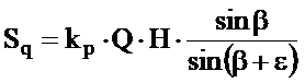
With application point equal to H/2 (being the diagram of the horizontal stresses constant for the entire height). In the above formula k_p is the coefficient of passive thrust calculated in the previous paragraph.

Cohesion

The cohesion determines an increase of resistance equal to:

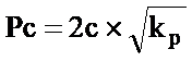
This increase is to be added directly to the main diagram of thrust.

Limit Equilibrium Method ( LEM )

The limit equilibrium method searches for solutions to the problem of verification or design which are compatible with only the static aspect of the problem. Basically we think in terms of equilibrium of a rigid body, without worrying about the kinematic congruence of displacements. The main calculation schemes which will be referred to are the following:

1. Cantilever bulkhead

2. Anchored bulkhead with a free end

3. Anchored bulkhead with a fixed end

Cantilever bulkhead: computation of limit embedment depth

For non-anchored bulkheads, the stability is ensured by the passive resistance of the soil which is located downstream of the bulkhead; the equilibrium of the moments with respect to the rotation center is obtained:

Where the symbols have the following meaning:

S_m= horizontal component of the active thrust

B_m= arm S_m with respect to O center of rotation

R_v= horizontal component of the passive resistance

B_v= arm R_v with respect to O center of rotation

Each term is a function of t, where t is the depth of the rotation center relative to the downstream reference plane (ground level downstream). The length needed to ensure the equilibrium to horizontal translation is achieved by increasing t as follows:

Figure 3: Diagram of reference for the calculation of bulkhead equilibrium

Safety coefficients on passive resistance

The embedment length d as above is determined relative to the limit condition of incipient collapse, through a coefficient F. It is possible to introduce a safety margin on the passive resistances; the reduction shall be carried out as follows:

Anchored bulkhead with free end: computation of the limit embedment depth

The stability of the work is also ensured by tie rods anchored on the bulkhead. To use the calculation scheme to free end, the bulkhead must be sufficiently short and rigid. The embedment length will be determined by imposing the equilibrium to the rotation about the origin of the tie rod indicated B1

Where the symbols have the following meaning:

S_m= horizontal component of active thrust

H= height of ground to support

t= calculated embedment depth

B_m= arm S_m with respect to the base of the bulkhead

P_m= ordinate of the anchor point of application upstream

R_v = horizontal component of the passive resistance

B_v = arm of R_v

Knowing t, are determined S_m and R_v and the relative stress of the anchor.

Safety factor F on passive resistances

The embedment length will be further increased in order to obtain safety margin in operating conditions using the safety coefficient F:

Anchored bulkhead with fixed end: computation of limit embedment depth

If the deeper section of the bulkhead does not move and does not rotate can be assimilated to a joint, in which case the bulkhead is defined with fixed end. A process developed by BLUM allows to obtain the embedment depth (t + t '), imposing the kinematic conditions of null displacements at the base of the work and at the origin of the anchor (B1), and the static conditions of moment and null shear at the base of the bulkhead. This leads to an equation of the 5^th degree (t + t ') which can be easily solved.

Safety coefficient F on resistances

To increase the safety factor were introduced, in the numerical developments, values of reduced passive resistances.

Finite Element Method (FEM)

The finite element method is the method that most of all it is based on solid theoretical and rational foundations. In fact all the method assumes that the problem is addressed taking into account both the static (and therefore the equilibrium of the problem) and the kinematics aspects (and therefore the consistency of the movements or better of deformations). In this approach the bulkhead is modeled as a set of beams, with continuity bond between them (beam elements) bound to the ground by elastic springs, whose stiffness is evaluated according to the elastic properties of the soil. The following figure shows schematically the model used for the finite element analysis:

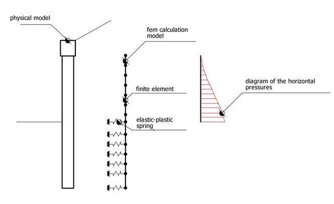
Figure 4: Schematic representation of a bulkhead with finite elements

Various aspects are pivotal in this calculation method. The following section shows the essential aspects.

Calculation of the Ks modulus

As mentioned previously, the ground is schematically shown with the springs of Ks stiffness applied on the nodes of the slices between the dredge line node and the end of embedment. The computation of the stiffness Ks was carried out on the basis of the foundations bearing capacity according to the following formula:

Where the symbols have the following meaning:

As= constant, calculated as As=C·(c·Nc+0.5·G·B·Ng)

Bs= coefficient function of depth Bs=C·G·Nq

Z= depth in question

C= 40 in the international system of units SI

n= π·tanφ

Nq= exp[n·(tan²(45° + φ/2)]

Nc= (Nq-1)·cotφ

Ng= 1.5·(Nq-1)·tanφ

Anchors\ The anchors are summarized as elastic elements, with cross section of area equal to A, modulus of elasticity E and the length L. For a segment of bulkhead of unitary width, the action of the anchors inclined at an angle β ισ:

Siphoning

The siphoning is a phenomenon that in an initial phase is localized to the foot of the bulkhead, and then rapidly extends in the neighborhood of the resistant volume. Occurs when, for a high hydrodynamic pressure or infiltration, are annulled the effective passive pressures, with the consequent loss of the soil resistance. Usually the safety factor Fsiph = 3.5-4 indicating with:

ic = critical hydraulic gradient

ie = hydraulic gradient in operating conditions

The safety margin is defined as the ratio between ic and ie, if ie\<ic the bulkhead is stable.

Uplift check for dredge line

In the case of a diaphragm driven into the ground, the presence of the water in positions such as to trigger a filtration motion involves the establishment of a filtration force which, if directed upwards, may cancel the weight of the soil which, in the absence of cohesion, it can be dragged by the water flow and affect the stability of the work. The phenomenon of dredge stability, similar to that of siphoning, has been faced for the first time by Terzaghi (1943). Unlike the siphoning, which is a localized phenomenon in the outlet point of the first flow line, the dredge uplift extends to a depth equal to bulkhead embedment depth for a width equal to half of that embedment.

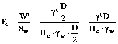
To simplify the problem of determining the actual results from porewater pressure at point A, it is assumed that the value of the overpressure to the foot of the diaphragm is constant over the length D/2 and equal to D/2 and equal to γ_wxH_c. H_c is used to determine the expression of the efflux gradient i_E:

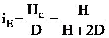
From which is obtained:

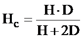
The filtration force S_w which tends to lift the block of soil involved is equal to:

The limit conditions of stability are reached when S_w equals the effective weight of the block, therefore, the dredge uplift safety factor is defined as the ratio between the effective weight of the block and the filtration force:

Sections check and reinforcement computation

The calculation of reinforcement and buckling and shear checks of the bulkhead subject to stresses N, M and T, are carried out on the most stressed section. The calculation stresses are obtained as the product between the stresses obtained from a linear meter calculation and the distance between the piles (or width of the baffles if the bulkhead is formed by septum):

Where M', M', T' represent the moment, the shear and the normal stress relative to a unitary strip of calculation while i is the distance between the piles to the bulkhead consisting of piles or micropiles (or width septa for the bulkhead formed by septa).