Traveltime curves

Objective of this step: to turn the first arrivals into time–distance curves and, by reading their slopes, decide how many layers the subsoil has. This is where the most important interpretative decision is taken.

Once the first arrivals have been picked on all the seismograms, move to the Traveltime curves tab: the software builds the curves automatically.

Cleaning up the view

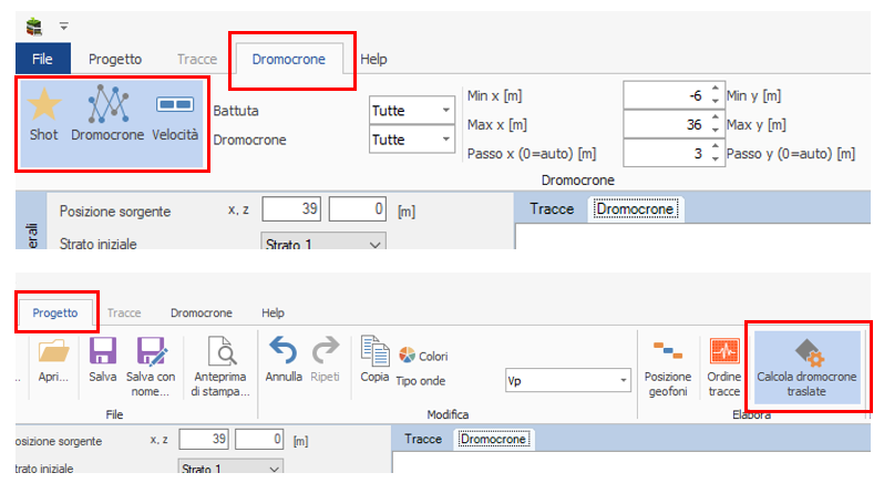
At the start the diagram is crowded. To be able to read it, temporarily deselect:

• shot — the polylines joining the time–distance points of each shot;
• velocity — the numerical labels on the segments;
• processed traveltime curves (phantomed traveltime curves) — the combination of the curves of all the shots.

Studying one curve at a time

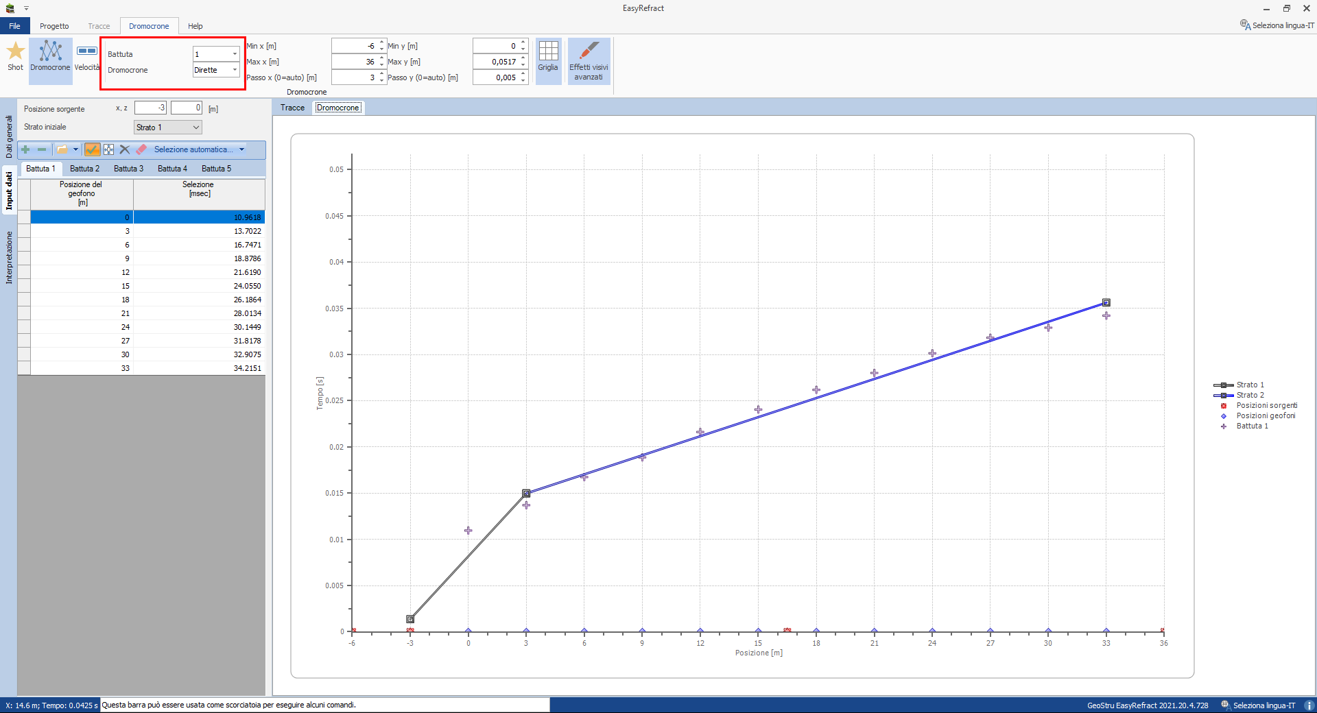
It is best to isolate one shot and one type of traveltime curve at a time, for example Shot 1 → Direct traveltime curve.

Direct or reverse depends on the shot

A shot placed at the start of the spread produces only direct traveltime curves; one placed at the tail only reverse ones. Asking for the reverse curve of Shot 1 will show nothing: this is not a malfunction.

Counting the layers from the slopes

Each straight segment of the curve corresponds to a material at constant velocity; each slope change (knee point) is a crossover point, that is the point at which a faster refracted wave takes over.

Read the curve starting from the origin:

1. the first segment, the steepest, is the direct wave (\(V_1\));
2. the next segment, flatter, is the first refracted wave → 1st refractor;
3. a possible third, even flatter segment → 2nd refractor;

and so on. Then apply the rule:

N layers ⇒ N−1 refractors

2 segments (direct + 1 refracted) ⇒ 1 refractor ⇒ 2 layers. 3 segments (direct + 2 refracted) ⇒ 2 refractors ⇒ 3 layers.

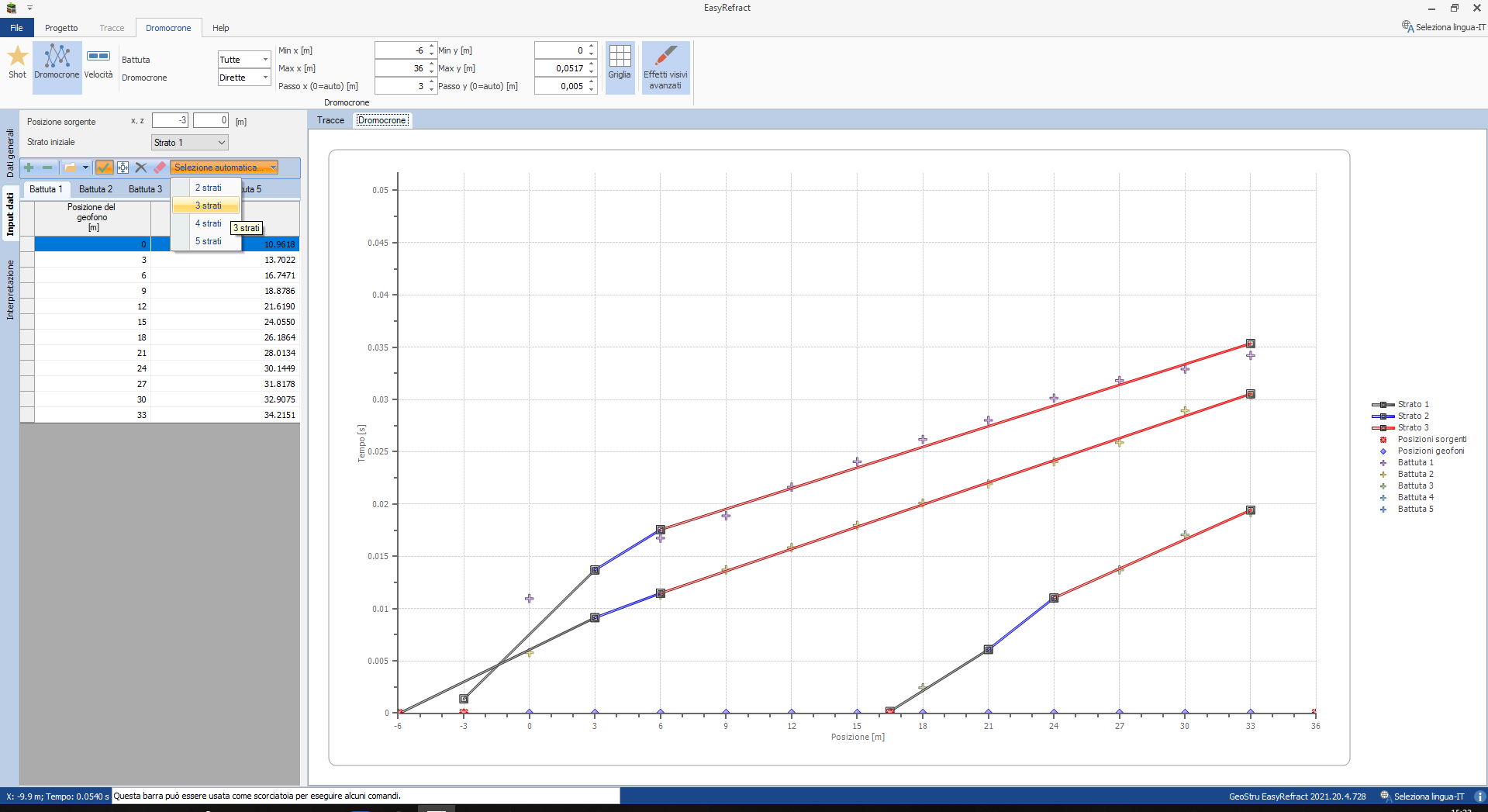
Set the number of layers from the Automatic selection window. The default value is arbitrary: it must be corrected on the basis of what you yourself read on the curves. When the number of layers is changed the traveltime curves are recalculated instantly, so you can try 2, 3 or 4 layers and see which hypothesis best describes the data.

Do not overdo the layers

Increasing the number of layers always produces an apparently better fit, but it introduces refractors that the data do not justify. Add a layer only if there is a recognisable straight segment on the traveltime curve to support it.

The knee points can be moved, inserted or deleted with the cursor (assign, move, insert point): the segment velocities are updated automatically at every change.

Phantomed traveltime curves

The Project → Calculate processed traveltime curves command recombines, using phantoming techniques, the traveltime curves of all the shots — direct ones on one side, reverse ones on the other — into a single curve for each refractor.

The phantomed curves represent only the refracted waves: the direct wave is excluded, because what matters is what travels along the refractors. They are therefore the most direct way of counting the refractors: one phantomed curve = one refractor.

With the traveltime curves correctly set, you can move on to the Data interpretation.