Shot points, data filtering and first arrivals

Objective of this step: to tell the software where each shot was fired from, to clean up the signal and finally to read the datum that really matters — the first arrival on each trace.

1. Source positions

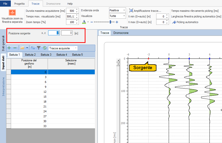
For each shot enter the Source position: fill in the x field (the position along the spread) and the z field (the elevation, if other than 0) and press Enter on the keyboard. A red star confirms the shot point on the diagram.

In the example with 12 geophones at 3 m spacing, the five shots are positioned at 0 m, 3 m, 22.5 m (central), 42 m and 45 m.

A mandatory step

Without the source position the software cannot calculate the source–geophone distances, and therefore no traveltime curve. It must be assigned to every shot, one by one.

2. Filtering (optional)

If the traces are affected by noise you can filter them: click on the funnel-shaped symbol. The Data filtering window opens.

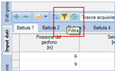
The software applies the Fourier transform to move from the space–time domain to the frequency domain, where the noise can be separated from the signal. Two filters are available:

• Low pass — lets the low frequencies through and cuts those above the threshold set (e.g. 200 Hz). Useful against high-frequency noise.
• Moving average — replaces each point with the average of N adjacent samples, smoothing the curve. The number of samples is always odd (3, 5, 7, 9…) because the average is assigned to the central point; the number of cycles can be increased to smooth further.

Press apply to see the effect immediately and repeat until the result is satisfactory, then ok.

Filter only as much as necessary

Filtering is meant to make the first arrival legible, not to make the trace "look nice". A filter that is too aggressive rounds off the wavefront and shifts the first arrival, falsifying the times.

3. Identifying the first arrivals (picking)

This is the most delicate step of the entire processing: the times you read here become the traveltime curves and, in the end, the shape of the refractors.

As you bring the cursor close to a trace, a line orthogonal to the time axis appears: by clicking at the point where you believe the first oscillation arrived, a red segment appears. Repeat for every geophone and for every shot.

Tools that make the picking reliable

• Show zoom on separate window — opens a window that magnifies the portion of trace under the cursor. It is the tool that allows the true first arrival to be distinguished from the noise preceding it: always use it.
• Zoom time [%] and Max. time displayed [ms] — expand the time scale so as to "open up" the oscillations.
• Traces amplification — if the signals are weak, increase the amplitude. By ticking Same amplification for all traces the value applies to all of them; if the amplified traces overlap to the point of becoming confused, tick Truncate trace amplitude.

Automatic picking is not enough

The Automatic picking command does exist, but the points it proposes are often not the real first arrivals. It should be used at most as a first draft: correct practice is to check and adjust manually, trace by trace, with the zoom window open. It is the step that requires the most patience and it is the one that determines the quality of the final result.

The consistency check to always carry out

As you move away from the source the first arrival must be progressively later: the red segments must lie along a regular, progressive trend. A point that "goes back" in time with respect to its neighbours is almost certainly a picking error or a trace contaminated by an external source of disturbance.

Once all the first arrivals have been picked, you can move on to the Traveltime curves.